COO-I-3. Metagenome assembly
Overview
Teaching: 0 min
Exercises: 60 minQuestions
How to assemble metagenomes from sequencing reads?
Objectives
Learn how to interpret basic assembly metrics, and compare the quality of different asseemblies
Metagenome assembly
The next step is to assemble these reads into longer sequences, taking advantage of the long overlaps one would expect in PacBio reads. The goal is to reconstruct individual genomes, or bins, representing the genomic content of different microbial species within the community. However, this process will require several steps. First, we will aim to identify contiguous sequences (contigs) from our reads, which will represent segments of the genomes. Metagenomic assembly is a computationally intense task, and many different tools exist that can do this, each with its own strengths and weaknesses. However, these analyses usually take a few hours. To bypass these long runtimes, two different assemblers have already been run, and you can find the result files in:
ls -l ~/data_bb3bcg20/Block1/COOI/Intermediate_files/Assembly
First assembler: miniasm
One of these assemblers, miniasm, is a relatively simple Overlap-Layout-Consensus wrapper. Take a look at the resulting Fasta file.
Exercise: Examine the miniasm metagenome assembly
- How many contigs did miniasm identify? - What is the size range of these contigs?
Solution
grep -c ">" ~/data_bb3bcg20/Block1/COOI/Intermediate_files/Assembly/miniasm/assembly_miniasm.fasta181 contigs.
seqkit stats ~/data_bb3bcg20/Block1/COOI/Intermediate_files/Assembly/miniasm/assembly_miniasm.fastaFrom ca. 13 kbp to ca. 3.6 Mbp
To get more information about the effect of the polishing steps, let’s take a better look at the contig length distribution. Let’s First, let’s get access to the correct files:
$ cd ~/GenomeBioinformatics/Block1/COO-I/Results
$ mkdir 03_assembly_miniasm
$ cd 03_assembly_miniasm
$ ln -s ~/data_bb3bcg20/Block1/COOI/Intermediate_files/Assembly/miniasm/ .
Exercise: Examine additional statistics related to the miniasm metagenome assembly
Write a python script that can read sequences from a fasta file, and prints the length of each contig in a separate line. Once you have done that, print that information to a file.
You can also simply use the python script in
~/data_bb3bcg20/bin/scripts/fasta_length.pyHowever, in order to use Python 3, you will need to use a python 3 environment. Do it by running:
$ python3.11And you can run the python script by doing (replace “fasta_file” with the name of the fasta file you want to analyse):
$ python ~/data_bb3bcg20/bin/scripts/fasta_length.py fasta_fileOnce you are done with this environment, you can go back to the previous environment by running
$ python2.7Now run your script and generate a file with the contig lengths called “assembly_miniasm.fasta.contigLengths”. Then run the following script:
$ perl ~/data_bb3bcg20/bin/scripts/stats.pl assembly_miniasm.fasta.contigLengthsSolution
$ python ~/data_bb3bcg20/bin/scripts/fasta_length.py assembly_miniasm.fasta | cut -f2 > assembly_miniasm.contigLengths
$ perl ~/data_bb3bcg20/bin/scripts/stats.pl assembly_miniasm.contigLengthsN = 181
Sum: 16216279
Mean: 89592.701657
Var: 139285829786.486
SD: 373210.168386
SE: 27740.493348
MAD: 12274
Min: 12926
p10: 18795
p25: 23405
Median: 34524
p75: 48697
p90: 98795
Max: 3611276
Second assembler: flye
A more sophisticated assembler has also been run: flye. You can find the results of this assembly, as well as intermediate assembly files, in the corresponding folder.
$ cd ~/GenomeBioinformatics/Block1/COO-I/Results
$ mkdir 04_assembly_flye
$ cd 04_assembly_flye
$ ln -s ~/data_bb3bcg20/Block1/COOI/Intermediate_files/Assembly/flye/ .
Exercise: Examine the flye assembly
How many contigs did flye identify? How does the distribution of contig sizes compare to the results by miniasm?
Solution
$ python3.11
$ python ~/data_bb3bcg20/bin/scripts/fasta_length.py flye/assembly.fasta | cut -f2 > assembly_flye.contigLengths
$ perl ~/data_bb3bcg20/bin/scripts/stats.pl assembly_flye.contigLengthsN = 267
Sum: 18428211
Mean: 69019.516854
Var: 75039714194.2722
SD: 273933.777023
SE: 16764.474901
MAD: 12884
Min: 6040
p10: 12091.5
p25: 18009.5
Median: 28323
p75: 51918
p90: 80768
Max: 3541958
To learn more about the assembly process, take a look at the assembly file within the folder “00-assembly”. How many contigs were generated at that point? How does this compare with the number of final contigs produced by flye?
Assembly metrics using Quast
To get better metrics for these assemblies, we can use Quast. This is a software that evaluates assembly quality by measuring metrics such as contig length, Nx values, read mapping, and gene annotation.
Like usual, explore the options available at Quast by doing:
quast -h
Exercise: Run Quast on the obtained assemblies
Solution
cd ~/GenomeBioinformatics/Block1/COO-I/Results/03_assembly_miniasm
quast -o quast_miniasm --pacbio ../../Data/Course_sample_metagenome.fastq.gz miniasm/assembly_miniasm.fasta
cd ~/GenomeBioinformatics/Block1/COO-I/Results/04_assembly_flye
quast -o quast_flye --pacbio ../../Data/Course_sample_metagenome.fastq.gz flye/assembly.fasta
Copy the Quast reports to your laptop and interpret the results. Check both the report.pdf file and the icarus viewer report (the latter will open in your browser).
Exercise: Interpret the Quast reports
What do the Nx distributions represent, and how do they differ between these two assemblies?
What percentage of reads map back to the assemblies? What percentage of reads are properly paired, and why do you think that is the case?
How do the GC% distributions differ, and what do you think they imply about the microbial community under study?
Solution
Nx plots represent the size of the shortest contig such that X% of the total assembly length is made up of contigs of that length or longer.
Properly paired: 0%. Because we do not have paired-end reads – this is not a trait of PacBio sequencing.
Assembly graphs using Bandage
In order to get a visual impression of how good the assembly is, it is always a good idea to take a look at the assembly graph. Assembly graphs are representations of contigs, including possible interactions between them. These graphs include contigs as coloured paths, and are drawn to scale. The contigs form loops, in such a way that their end-points link to other parts of the assembly for which some information in the data indicates possible, but not clear, assembly paths. One such example can be seen in the image below, from the software Bandage:
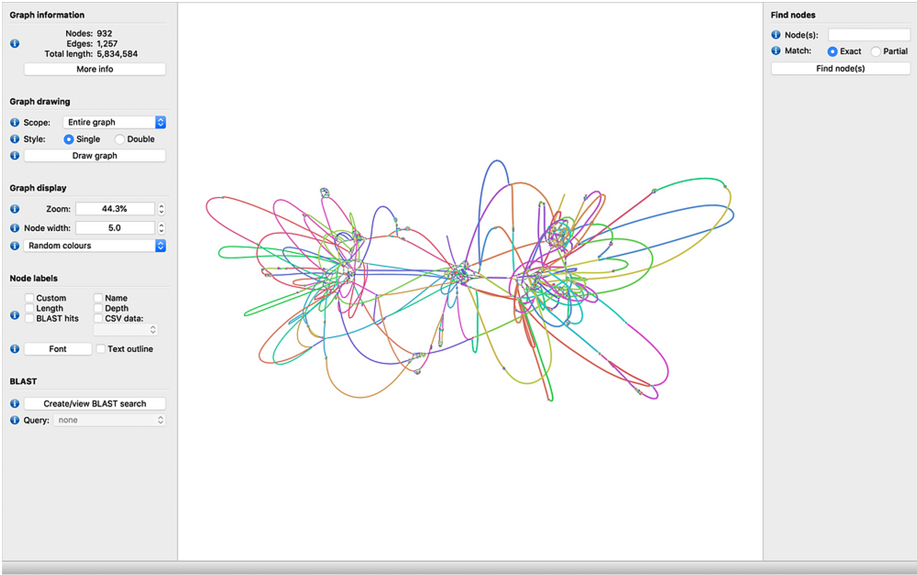
Perform this analysis in your own laptop, for the two assemblies we are inspecting. Download the software from their website (https://rrwick.github.io/Bandage/) and open it. Download the assembly graphs (“.gfa” files) using “scp” like before. Load one of the assembly graphs into Bandage and click on “Draw graph”. If Bandage does not work for you, feel free to take the corresponding Intermediate file. Do this for both assemblies and compare the results. What do you see? What is your impression of these assemblies based on the graphs?
Key Points